How Much Sun? Building the Dataset Behind the Model
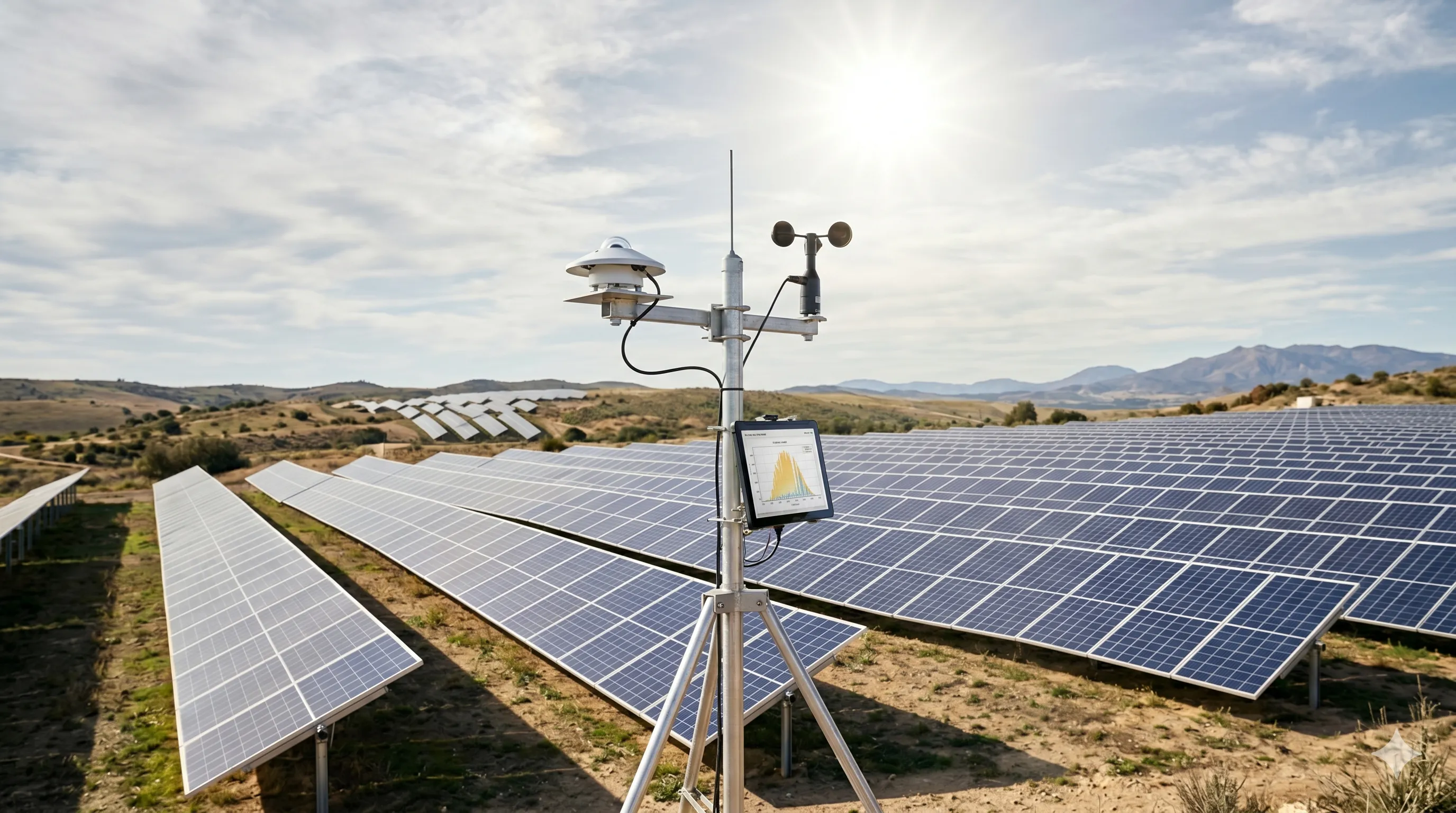
Project Finance, in Python, a three-part series. Part 1 · What a Solar Farm Is Worth · Part 2 · How Much Sun? (this post) · Part 3 · A Thousand Futures
In Part 1 I built a project finance model for a solar plant and found its returns hang almost entirely on one number: the resource, how much sunlight the site actually receives. The model treated that as a fixed assumption: 1,800 equivalent hours, every year, forever.
The whole point of this series is to stop pretending. To replace that single number with an honest range of possibilities, I need to understand how sunlight really behaves at a real location, not just its average, but its variability (how much it swings) and its persistence (whether bad days cluster together). And before you can model something, you have to measure it. This post is about building that measurement.
The problem: sunlight is two things at once
Stand outside on any given afternoon and the amount of sun hitting the ground is the product of two completely different forces.
The first is astronomy, and it is perfectly predictable. Given a latitude, a longitude, and a timestamp, physics tells you exactly how much solar energy would reach the ground if the sky were flawlessly clear. It’s higher at noon than at dawn, higher in June than December, higher in Seville than in Scotland. There is zero uncertainty here, we’ve known the geometry of the solar system for centuries. This is the clear-sky irradiance: the perfect score the sky could achieve.
The second force is weather (clouds, haze, dust) and it is pure randomness. It can only ever subtract from the perfect score, never add to it.
The orange envelope above is the deterministic clear-sky signal across a year, smooth, seasonal, knowable. The jagged blue line is what was actually measured: the clear-sky maximum, with weather taking bites out of it. Separating these two is the central trick of the whole dataset, because only one of them is uncertain, and uncertainty is the thing I’m trying to model.
Step 1: the perfect score, from astronomy
The clear-sky irradiance comes from pvlib, an open-source solar library. You hand it a location and a list of timestamps and it returns the theoretical irradiance for every hour: GHI (total light on a flat surface), DNI (the direct beam), and DHI (diffuse, scattered sky-light). For this project the site is in southern Spain near Badajoz, sunny, flat, the kind of place these plants actually get built:
loc = Location(38.812821, -6.521058, tz="UTC")     # near Badajoz, Spain
times = pd.date_range("2015-01-01", "2026-01-01", freq="1h", tz="UTC")
clearsky = loc.get_clearsky(times)   # GHI / DNI / DHI for every hour, 11 years
That’s the deterministic backbone, eleven years of “what a clear sky would deliver”, computed from nothing but orbital mechanics.
Step 2: what actually happened, from space
For the measured irradiance I pulled NASA POWER data, a satellite-derived record of the irradiance and cloud cover that genuinely occurred at those coordinates over the same eleven years. (Satellites are how you get a consistent, gap-free history for a site that never had a weather station on it, which is most sites.) Now each hour has two numbers side by side: what the sky could have delivered, and what it did.
Step 3: the Clear-Sky Index
Dividing one by the other collapses both into a single, beautifully normalised quantity, the Clear-Sky Index (CSI):
A CSI of 1.0 means a flawless day, the ground got everything astronomy promised. A CSI of 0.3 means heavy cloud stole 70% of it. By dividing out the clear-sky signal, the CSI throws away the predictable seasonal-and-daily cycle and keeps only the weather randomness, exactly the quantity I want to model.
That little (here, a constant of 0.5) is a practical fix, and it’s the kind of detail that separates a model that works from one that explodes. At dawn and dusk both irradiances approach zero, and dividing a tiny number by a tiny number gives numerical nonsense, the naïve ratio spikes wildly. Adding a small constant to top and bottom keeps the index stable through those moments:
csi = np.clip((ghi_measured + 0.5) / (ghi_clearsky + 0.5), 0, 1)To smooth out the hour-by-hour noise I aggregate to daily totals before taking the ratio, one CSI value per day, 4,000-odd days of weather distilled into a single clean series.
What the data says: southern Spain is relentlessly sunny
With eleven years of daily CSI in hand, the distribution tells the story:
This is not a bell curve, and that matters. The average daily CSI is 0.85, but the median is 0.95, and nearly half of all days land in the top bucket, near-perfectly clear. The distribution is heavily left-skewed: piled up against the 1.0 ceiling, with a long thin tail of genuinely bad days trailing off to the left.
In plain terms: at this site, a typical day is excellent, and the risk isn’t that sun is usually scarce, it’s the occasional run of cloudy weather, and the seasonal pattern underneath it. Winter months carry a noticeably fatter low-CSI tail than summer; the bad days aren’t spread evenly through the year, they bunch up in the dark months.
The two properties that matter for risk
Squint at that histogram and the data is quietly telling me two things I’ll need in Part 3.
One: the shape. Whatever model I fit has to reproduce this lopsided, skewed-toward-1.0 distribution, a symmetric bell curve would badly misrepresent it, overstating the bad days and understating how often the sky is perfect. A bounded [0, 1] quantity with a skew like this is a textbook case for a Beta distribution.
Two: the memory. Weather is persistent, a cloudy day tends to be followed by another cloudy day, because weather systems take days to pass. The CSI series isn’t a fresh independent dice-roll each morning; today’s value depends on yesterday’s. If I were to ignore that and just draw random days independently from the histogram, I’d scatter the bad days evenly and systematically understate the risk of a genuinely bad month, the cloudy week that drags a whole year’s production down. Capturing that memory is a job for a Markov chain.
There’s a second variable lurking too. The plant’s revenue isn’t just energy × constant, it’s energy × price, and the merchant electricity price has its own messy, volatile history. That history is the other half of the dataset, and it has a twist that completely reshapes the project’s economics. I’ll save it for the next post, where the data finally gets put to work.
From a clean dataset to a thousand futures
This post produced something deliberately unglamorous: a tidy table of clear-sky irradiance, measured irradiance, and cloud cover, eleven years long. No returns, no IRR, no charts of money. But it’s the foundation everything else stands on, because a stochastic model is only as honest as the data it’s calibrated to, and now I have a faithful, normalised picture of how the sky behaves at this exact spot on Earth.
In Part 3 this becomes the engine: I’ll fit a Markov-chain-plus-Beta model to that CSI distribution to capture both its shape and its memory, fit a second model to the electricity price, and then simulate a thousand different 30-year futures, feeding each one through the project finance model from Part 1 to turn a single deterministic IRR into a full probability distribution of returns.
→ Continue to Part 3 · A Thousand Futures: Monte Carlo Risk for a Solar Project
Notes, assumptions & further work
Key assumptions. A single site near Badajoz (lat 38.81, lon −6.52), 2015–2026; clear-sky irradiance from pvlib; measured irradiance and cloud cover from the NASA POWER satellite-reanalysis dataset; Clear-Sky Index defined as , clipped to and aggregated to daily totals.
Simplifications. NASA POWER is satellite-derived reanalysis, not a ground station, it carries its own bias and uncertainty, and a real bankable resource assessment would calibrate against on-site measurements and cross-check sources like PVGIS or a TMY file. The analysis uses GHI only (horizontal), leaving the tilt/orientation gain to a transposition factor later; the +0.5 constant in the CSI is a pragmatic fix for the sunrise/sunset singularity; the choice of clear-sky model affects the index; daily aggregation hides intra-day variability; and no long-term climate trend (or its effect on future resource) is removed or modelled.
Where it could go further. Calibrate the satellite series against ground data and quantify its uncertainty; cross-validate with PVGIS/TMY; model plane-of-array irradiance directly rather than via a flat transposition factor; examine inter-annual trends and climate-change drift in the resource; and test how sensitive the downstream returns are to the CSI definition itself.
Data pipeline and notebooks on GitHub. Built with pvlib and the NASA POWER dataset.
Last modified: 17 Jun 2026