Finite Element Method

The finite element method is a numerical technique used to solve complex engineering and physical problems. It is a powerful tool that allows for the accurate prediction of the behavior of a system under a wide range of conditions, making it an essential tool for engineers and scientists working in fields such as structural analysis, fluid dynamics, and electromagnetics.

By the end of this tutorial you will be able to implement the finite element method in Python and apply it to solve a simple 2D structural problem.

All the code can be found here.

Introduction

The Finite Element Method works by dividing a physical space into different elements and applying the governing equations to each element. This is very useful for complex geometries or boundary conditions where obtaining an analytical expression is not feasible.

Although FEM can be applied to many different physical problems, it is most commonly used in structural analysis. We will develop the FEM for structural analysis in 2D.

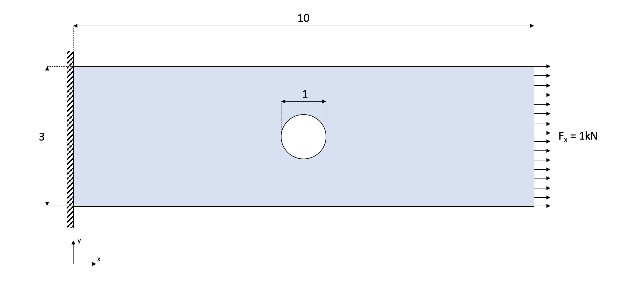
In this example the structural case will be a 2D rectangular plate ( $3\text{m} \times 10\text{m}$ ) with a hole of $1\text{m}$ diameter, fixed on one side and subjected to a constant tension force of $1\,\text{kN}$ on the opposite side:

2D plate with a circular hole under tension

To simplify the calculations, 3-node triangular elements will be used.

The main equation in the FEM for structural analysis is:

$\textbf{K} \textbf{d} = \textbf{F}$

Where $\textbf{d}$ is the displacement vector, $\textbf{F}$ is the force vector, and $\textbf{K}$ is the stiffness matrix. For the rest of the tutorial the force vector will be expressed as the sum of the external forces ( $\textbf{f}$ ) and the reaction forces ( $\textbf{r}$ ):

$\textbf{K} \textbf{d} = \textbf{f} + \textbf{r}$

While displacements and forces are intuitive to understand, the stiffness matrix is more abstract. It can be understood as the resistance to deformation — analogous to the spring constant ( $k$ ) in Hooke’s law:

Requirements

pip install numpy pygmsh gmsh pyglet

import numpy as np
from math import *
import drawMesh
import pygmsh
import gmsh

Mesh

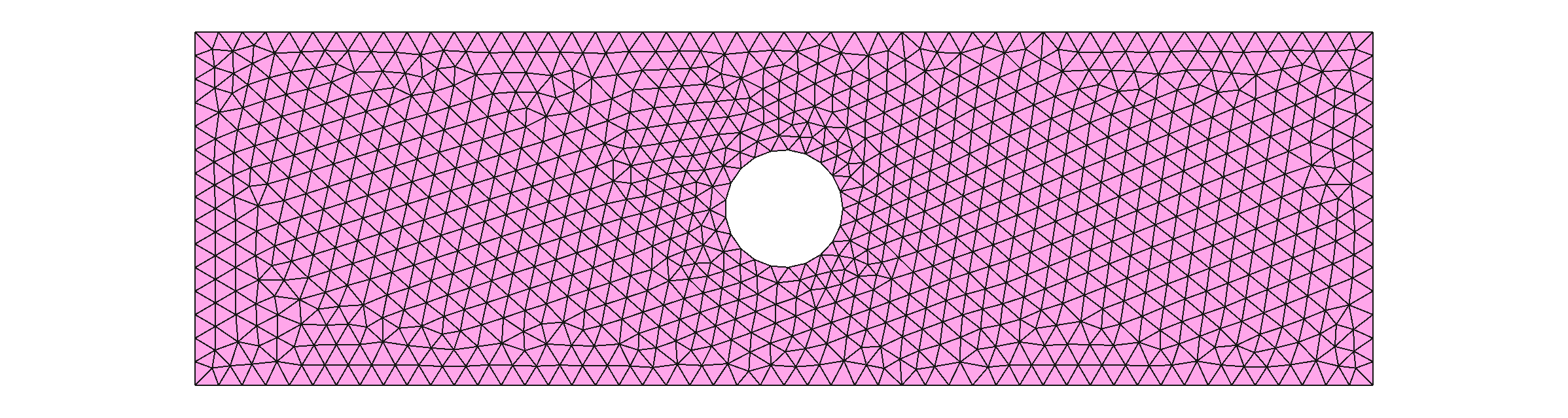
Splitting the geometry into elements and nodes can be done manually, but it becomes exponentially difficult for complex geometries and finer mesh resolutions. We use gmsh, a powerful meshing tool.

The mesh resolution is defined in resolution. Lower values create more elements and give better results at higher computational cost.

gmsh.initialize()
rect_width, rect_length = 3.0, 10.0
resolution = 0.1

geom = pygmsh.geo.Geometry()

circle = geom.add_circle([5, 1.5, 0], radius=0.5, mesh_size=resolution * 0.5, make_surface=False)

rect = geom.add_polygon(
    [
        [0.0,           0.0,          0],
        [0.0,           rect_width,   0],
        [rect_length,   rect_width,   0],
        [rect_length,   0.0,          0],
    ],
    mesh_size=resolution,
    holes=[circle]
)

mesh = geom.generate_mesh(dim=2)
geom.__exit__()

The resulting mesh looks like this:

Node

The Node class represents a node in the mesh. It stores the node’s coordinates, external forces, reaction forces, and displacements.

class Node:

    def __init__(self, id, x, y):
        self.id = id
        self.x, self.y = x, y
        self.fx, self.fy = 0.0, 0.0
        self.rx, self.ry = 0.0, 0.0
        self.dx, self.dy = None, None

    @property
    def dfix(self):
        return self.dx == 0.0 and self.dy == 0.0

    @property
    def externalForce(self):
        return self.fx != 0.0 or self.fy != 0.0

    def __eq__(self, obj):
        return (self.x == obj.x) and (self.y == obj.y)

Element

Each element contains three nodes. The nodes are ordered counter-clockwise in orderCounterClock(). Each element stores a stress ( $\vec{\sigma}$ ) and strain ( $\vec{\varepsilon}$ ) attribute:

\vec{\sigma} = \begin{bmatrix} \sigma_{xx}\\ \sigma_{yy}\\ \sigma_{xy} \end{bmatrix} \qquad \vec{\varepsilon} = \begin{bmatrix} \varepsilon_{xx}\\ \varepsilon_{yy}\\ \gamma_{xy} \end{bmatrix}

class Element:

    maxColorVal = -9.9e19
    minColorVal = 9.9e19
    colorFunc = lambda x: x

    def __init__(self, id, nodes):
        self.id = id
        self.nodes = self.orderCounterClock(nodes)
        self.stress = None
        self.strain = None
        self.colorVal = 0
        self.getArea()

    def getde(self):
        de_ = []
        for n in self.nodes:
            de_.append(n.dx)
            de_.append(n.dy)
        self.de = np.array(de_)
        return self.de

    def getColor(self):
        try:
            x_ = float(self.colorVal - Element.minColorVal) / (Element.maxColorVal - Element.minColorVal)
        except ZeroDivisionError:
            x_ = 0.5
        x = Element.colorFunc(x_)
        blue  = int(255 * min(max(4 * (0.75 - x), 0.), 1.))
        red   = int(255 * min(max(4 * (x - 0.25), 0.), 1.))
        green = int(255 * min(max(4 * fabs(x - 0.5) - 1., 0.), 1.))
        return (red, green, blue)

    def getArea(self):
        x1, y1 = self.nodes[0].x, self.nodes[0].y
        x2, y2 = self.nodes[1].x, self.nodes[1].y
        x3, y3 = self.nodes[2].x, self.nodes[2].y
        result = 0.5 * ((x2*y3 - x3*y2) - (x1*y3 - x3*y1) + (x1*y2 - x2*y1))
        if result == 0:
            result = 1e-20
        self.area = result
        return result

    def getBe(self):
        x1, y1 = self.nodes[0].x, self.nodes[0].y
        x2, y2 = self.nodes[1].x, self.nodes[1].y
        x3, y3 = self.nodes[2].x, self.nodes[2].y
        B = (0.5 / self.area) * np.array([
            [(y2-y3),    0,       (y3-y1),    0,       (y1-y2),    0      ],
            [0,       (x3-x2),    0,       (x1-x3),    0,       (x2-x1)   ],
            [(x3-x2), (y2-y3),    (x1-x3), (y3-y1),    (x2-x1), (y1-y2)  ],
        ], dtype=np.float64)
        self.Be = B
        return B

    def getKe(self, D):
        Bie = self.getBe()
        Ke = self.area * np.matmul(Bie.T, np.matmul(D, Bie))
        self.Ke = Ke
        return Ke

    def orderCounterClock(self, nodes):
        p1, p2, p3 = nodes[0], nodes[1], nodes[2]
        val = (p2.y - p1.y) * (p3.x - p2.x) - (p2.x - p1.x) * (p3.y - p2.y)
        nodes_ = nodes.copy()
        if val > 0:
            nodes[1] = nodes_[0]
            nodes[0] = nodes_[1]
        assembly = []
        for n in nodes:
            assembly.append(int(n.id * 2))
            assembly.append(int(n.id * 2) + 1)
        self.assembly = assembly
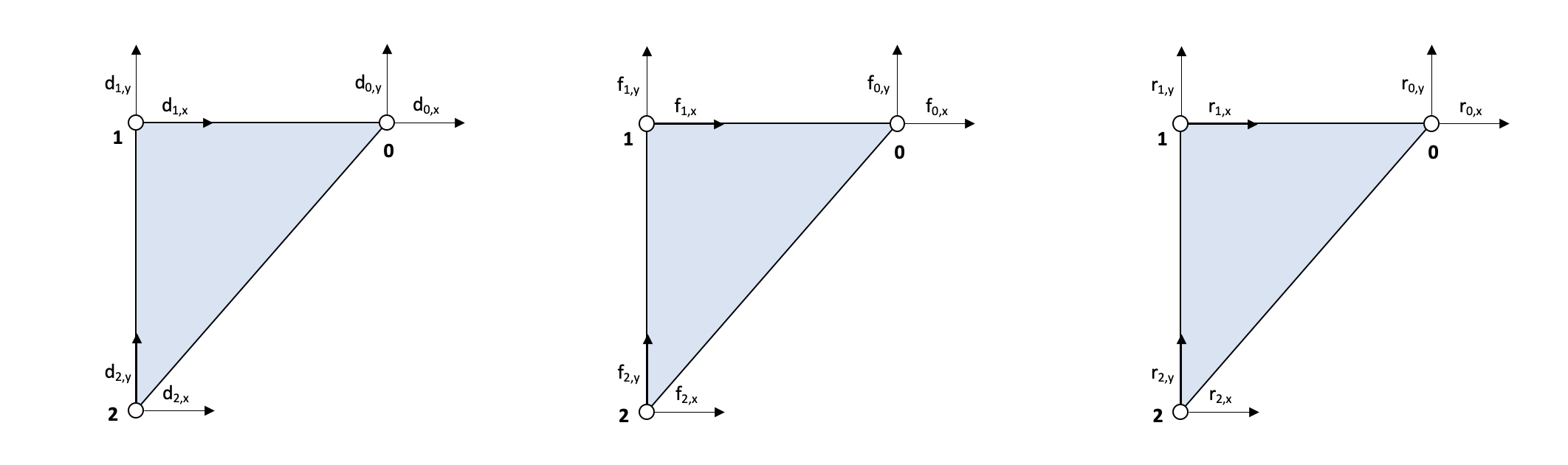
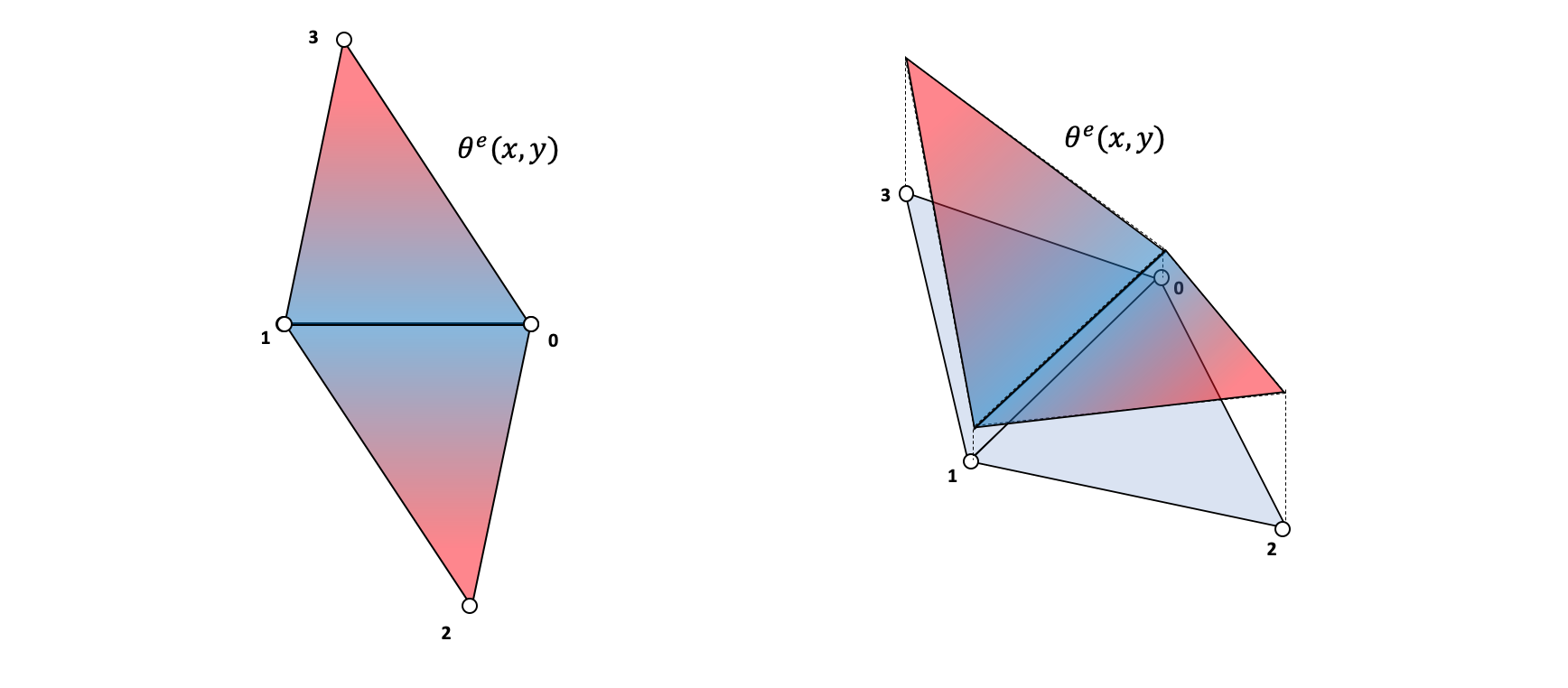
        return nodes

It is important to distinguish between global and local variables. Element numbers are denoted with a superscript and node numbers with a subscript. For example, the local point 0 of element 4 is denoted $P_0^{(4)}$ . Note that $P_0^{e} \neq P_0$ .

The force-displacement equation for an element is $\mathbf{K^e} \mathbf{d^e} = \mathbf{f^e} + \mathbf{r^e}$ , where:

\mathbf{d^e} = \begin{bmatrix} d_{0,x}^e \\ d_{0,y}^e \\ d_{1,x}^e \\ d_{1,y}^e \\ d_{2,x}^e \\ d_{2,y}^e \end{bmatrix} \qquad \mathbf{K^e} = \begin{bmatrix} k_{00} & k_{01} & k_{02} & k_{03} & k_{04} & k_{05} \\ k_{10} & k_{11} & k_{12} & k_{13} & k_{14} & k_{15} \\ k_{20} & k_{21} & k_{22} & k_{23} & k_{24} & k_{25} \\ k_{30} & k_{31} & k_{32} & k_{33} & k_{34} & k_{35} \\ k_{40} & k_{41} & k_{42} & k_{43} & k_{44} & k_{45} \\ k_{50} & k_{51} & k_{52} & k_{53} & k_{54} & k_{55} \end{bmatrix}

The element stiffness matrix is obtained from the weak form of the elasticity problem:

\mathbf{K^e} = \int_{\Omega}(\mathbf{B^e})^T \mathbf{D} \, \mathbf{B^e} \, d\Omega

The Hookean matrix $\mathbf{D}$ relates strain and stress taking into account the material properties. The matrix $\mathbf{B^e}$ relates the displacements at the nodes to the gradient of the displacement function $\theta^e(x,y)$ :

$\nabla \theta^e = \mathbf{B}^e \mathbf{d}^e$

The displacement function interpolates the node displacements across the element space, such that at each node the function matches the displacement.

Displacement function interpolation across an element

For triangular elements, the $\mathbf{B^e}$ matrix is:

\mathbf{B^e} = \frac{1}{2 A^e} \begin{bmatrix} (y_1^e - y_2^e) & 0 & (y_2^e - y_0^e) & 0 & (y_0^e - y_1^e) & 0 \\ 0 & (x_2^e - x_1^e) & 0 & (x_0^e - x_2^e) & 0 & (x_1^e - x_0^e) \\ (x_2^e - x_1^e) & (y_1^e - y_2^e) & (x_0^e - x_2^e) & (y_2^e - y_0^e) & (x_1^e - x_0^e) & (y_0^e - y_1^e) \end{bmatrix}

Since $\mathbf{B^e}$ is constant along the element surface, we can simplify the stiffness matrix to:

$\mathbf{K^e} = (\mathbf{B^e})^T \mathbf{D} \, \mathbf{B^e}$

Preprocessing

Extracting mesh data

The mesh contains points and cells data. Each row in cells contains the indices of the three points forming that element.

\textbf{cells} = \begin{bmatrix} P_0^{(0)} & P_1^{(0)} & P_2^{(0)} \\ P_0^{(1)} & P_1^{(1)} & P_2^{(1)} \\ \vdots & \vdots & \vdots \end{bmatrix} \qquad \textbf{points} = \begin{bmatrix} P_0 \\ P_1 \\ \vdots \end{bmatrix} \qquad P_i = \begin{bmatrix} x_i & y_i \end{bmatrix}

meshCells = mesh.cells[1].data - np.full(np.shape(mesh.cells[1].data), 1, dtype=np.uint64)
meshPoints = mesh.points[1:]

nodes = [Node(i, point[0], point[1]) for i, point in enumerate(meshPoints)]
elements = []

for i, cell in enumerate(meshCells):
    elements.append(Element(id=i, nodes=[nodes[i] for i in cell]))

Material properties

The Hookean matrix $\mathbf{D}$ can be calculated from the Young’s modulus ( $E$ ) and Poisson’s ratio ( $\nu$ ):

\mathbf{D} = \frac{E}{1-\nu^2} \begin{bmatrix} 1 & \nu & 0 \\ \nu & 1 & 0 \\ 0 & 0 & \frac{1-\nu}{2} \end{bmatrix}

Using the material properties of steel:

v = 0.28       # Poisson ratio
E = 200.0e9    # Young's modulus (Pa)

D = (E / (1 - v**2)) * np.array([
    [1, v, 0],
    [v, 1, 0],
    [0, 0, (1 - v) / 2],
])

Boundary conditions

for i, node in enumerate(nodes):
    if node.x == rect_length:           # Right side: apply tension
        node.fx = 1.0e3
    elif node.x == 0.0:                 # Left side: fix displacement
        node.dx, node.dy = 0.0, 0.0
        node.rx, node.ry = None, None   # Reaction forces are unknowns

Matrix assembly

The global stiffness matrix is the sum of all element stiffness matrices:

$\mathbf{K} = \sum_{i=0}^{N_{el}} \mathbf{\hat{K}^e}$

Note that $\mathbf{\hat{K}^e} \neq \mathbf{K^e}$ : the local matrix $\mathbf{K^e}$ has shape $(6 \times 6)$ while the global one $\mathbf{\hat{K}^e}$ has shape $(2N_n \times 2N_n)$ . The assemblyK function maps each element’s local stiffness matrix into the global one:

def assemblyK(K, Ke, nodeAssembly):
    for i, t in enumerate(nodeAssembly):
        for j, s in enumerate(nodeAssembly):
            K[t][s] += Ke[i][j]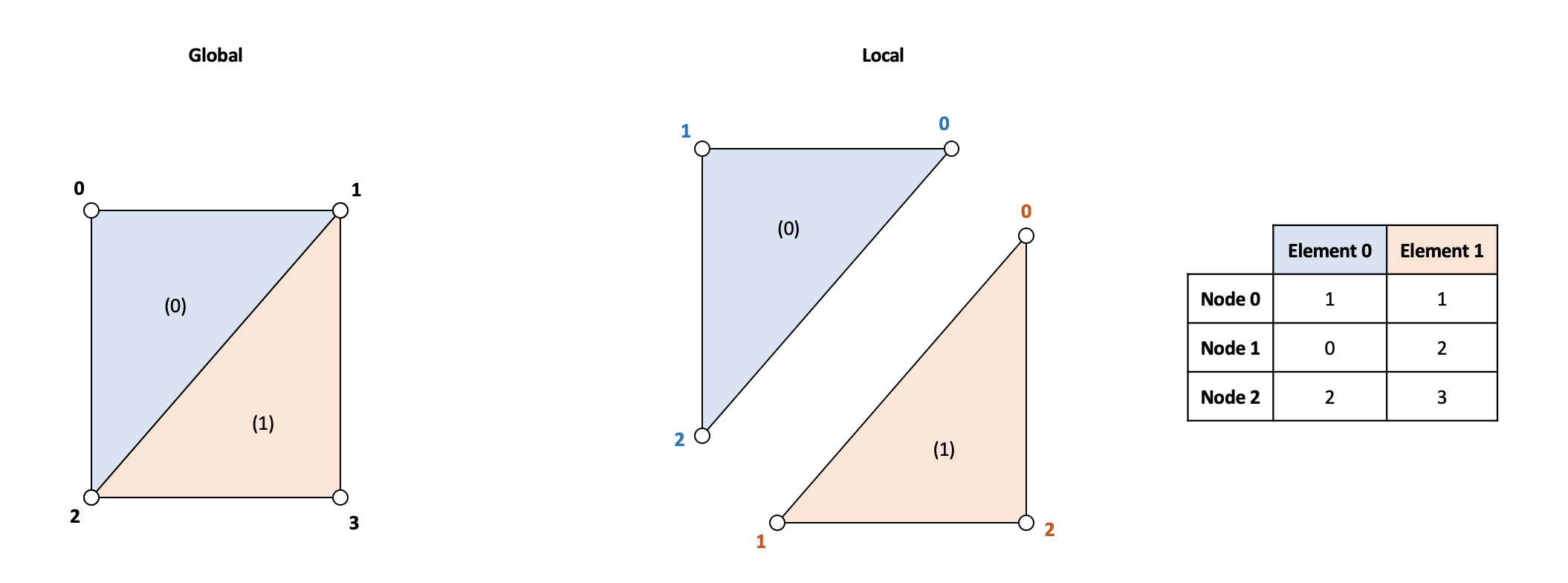

Node assembly mapping from local to global stiffness matrix

Nnodes = len(nodes)
K = np.zeros((Nnodes * 2, Nnodes * 2))

for e in elements:
    Ke = e.getKe(D)
    assemblyK(K, Ke, e.assembly)

Build the force, reaction, and displacement vectors:

f = np.zeros((int(2 * Nnodes), 1))
d = np.full((int(2 * Nnodes), 1), None)
r = np.full((int(2 * Nnodes), 1), None)

rowsrk, rowsdk = [], []

for i, node in enumerate(nodes):
    ix, iy = int(i * 2), int(i * 2) + 1
    f[ix], f[iy] = node.fx, node.fy
    d[ix], d[iy] = node.dx, node.dy
    r[ix], r[iy] = node.rx, node.ry
    if node.dx is None:
        rowsrk.append(ix)
    else:
        rowsdk.append(ix)
    if node.dy is None:
        rowsrk.append(iy)
    else:
        rowsdk.append(iy)

Solver

We partition the system of equations by known and unknown variables. For unknowns, we separate $\mathbf{d_U}$ (unknown displacements) and $\mathbf{f_U}$ (unknown reaction forces) from their known counterparts. The system becomes:

\begin{bmatrix} \mathbf{K_{A}} & \mathbf{K_{AB}} \\ \mathbf{K_{AB}^T} & \mathbf{K_{B}} \end{bmatrix} \begin{bmatrix} \mathbf{d_K} \\ \mathbf{d_U} \end{bmatrix} = \begin{bmatrix} \mathbf{f_U} \\ \mathbf{f_K} \end{bmatrix}

Since the known displacements are zero, this simplifies to:

$\mathbf{d_U} = \mathbf{K_B}^{-1} \mathbf{f_K} \qquad \mathbf{f_U} = \mathbf{K_A} \mathbf{d_U}$

KB = np.zeros((len(rowsrk), len(rowsrk)))
KA = np.zeros((len(rowsdk), len(rowsrk)))

fk = np.array([r[i] for i in rowsrk]) + np.array([f[i] for i in rowsrk])
dk = np.array([d[i] for i in rowsdk])

for i in range(np.shape(KB)[0]):
    for j in range(np.shape(KB)[1]):
        KB[i][j] = K[rowsrk[i]][rowsrk[j]]

for i in range(np.shape(KA)[0]):
    for j in range(np.shape(KA)[1]):
        KA[i][j] = K[rowsdk[i]][rowsrk[j]]

du = np.matmul(np.linalg.inv(KB), fk)
fu = np.matmul(KA, du)

Postprocessing

Assign the solved displacements back to the nodes:

d_total = d.copy()
for i, d_solve in zip(rowsrk, du):
    d_total[i] = d_solve

for i, n in enumerate(nodes):
    ix, iy = int(i * 2), int(i * 2) + 1
    n.dx = d_total[ix][0]
    n.dy = d_total[iy][0]

Von Mises stress

The von Mises equivalent stress is a good predictor for plastic yielding:

$\sigma_v = \sqrt{\sigma_{xx}^2 + \sigma_{yy}^2 + 3\sigma_{xy}^2 - \sigma_{xx}\sigma_{yy}}$

def calculateVonMises(sx, sy, sxy):
    return sqrt(sx**2 + sy**2 + 3 * (sxy**2) - sx * sy)

Calculate strains and stresses for each element using Hooke’s generalized expression:

$\varepsilon^e = \mathbf{B}^e \mathbf{d}^e \qquad \sigma^e = \mathbf{D} \varepsilon^e$

Element.colorFunc = lambda x: x  # Can be changed to exp(-x) for log scale

for i, element in enumerate(elements):
    de = element.getde()
    strain_e = np.matmul(element.Be, de)
    stress_e = np.matmul(D, strain_e)
    element.strain = strain_e
    element.stress = stress_e
    element.colorVal = calculateVonMises(element.stress[0], element.stress[1], element.stress[2])
    if element.colorVal > Element.maxColorVal:
        Element.maxColorVal = element.colorVal
    if element.colorVal < Element.minColorVal:
        Element.minColorVal = element.colorVal

render = drawMesh.MeshRender()
render.legend = True
render.autoScale = True
render.deform_scale = 1.0e5
render.legendTitle = 'von-mises (Pa)'
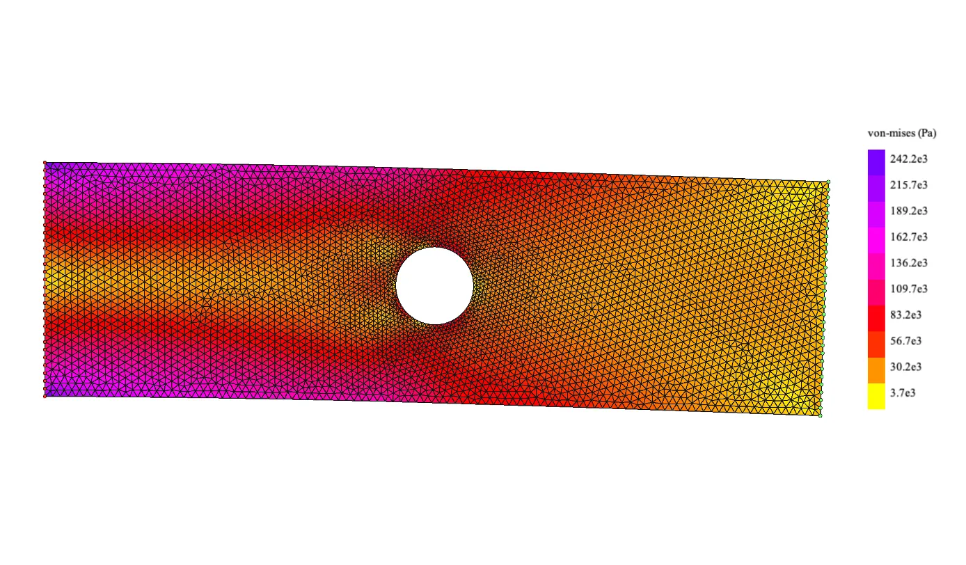
render.drawElements(elements)

Results

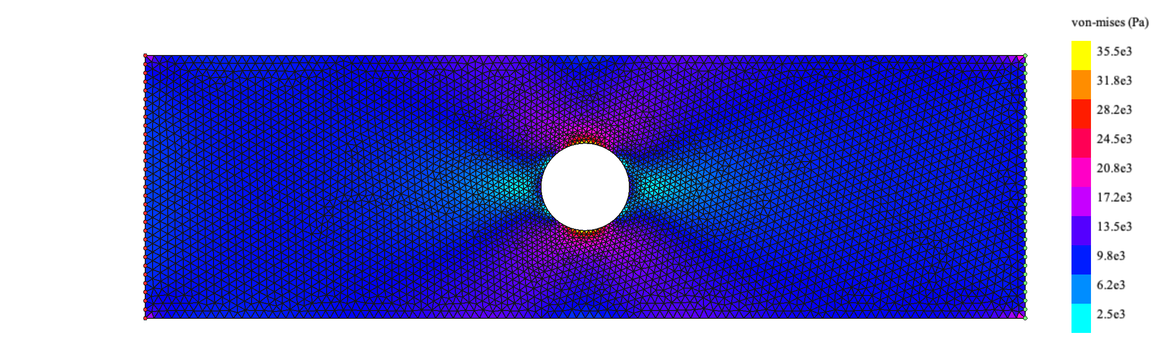
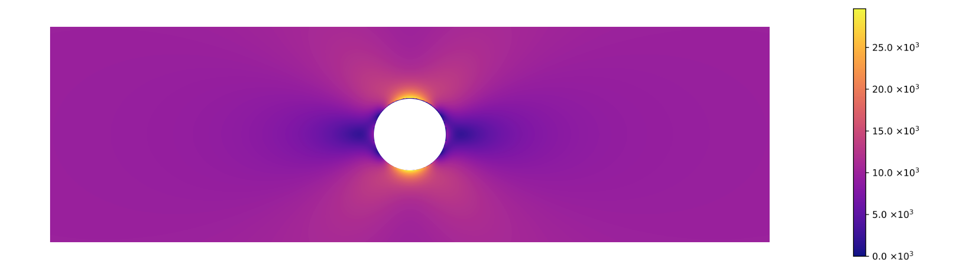
Applying horizontal tension (x-direction):

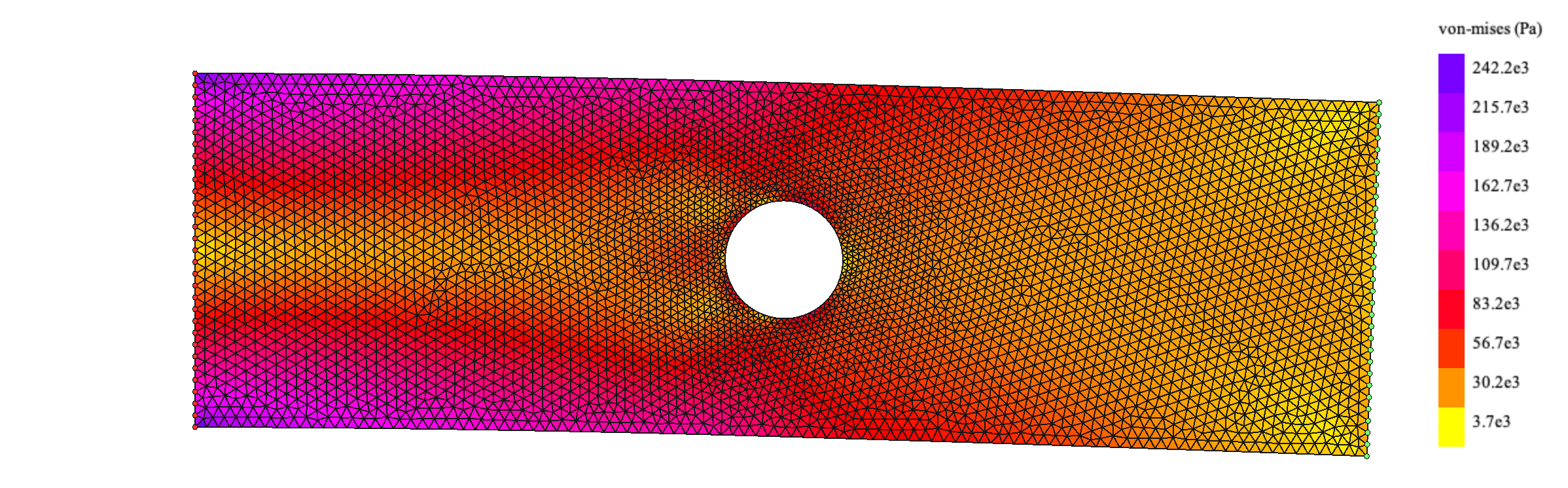
Applying vertical force (y-direction) instead:

Von Mises stress — vertical load (log scale)

Analytical validation

The classic problem of a plate with a hole under tension has a known analytical solution. In polar coordinates, with plate half-width $\gg R$ and applied stress $\sigma_t$ :

$\sigma_r(r, \theta) = \frac{\sigma_t}{2}\left(1 - \frac{R^2}{r^2}\right) + \frac{\sigma_t}{2}\left(1 + 3\frac{R^4}{r^4} - 4\frac{R^2}{r^2}\right)\cos(2\theta)$

$\sigma_\theta(r, \theta) = \frac{\sigma_t}{2}\left(1 + \frac{R^2}{r^2}\right) - \frac{\sigma_t}{2}\left(1 + 3\frac{R^4}{r^4}\right)\cos(2\theta)$

$\tau_{r\theta}(r, \theta) = -\frac{\sigma_t}{2}\left(1 - 3\frac{R^4}{r^4} + 2\frac{R^2}{r^2}\right)\sin(2\theta)$

Plotting the analytical von Mises stress with the same parameters:

The FEM results match the analytical solution closely, which validates the implementation.